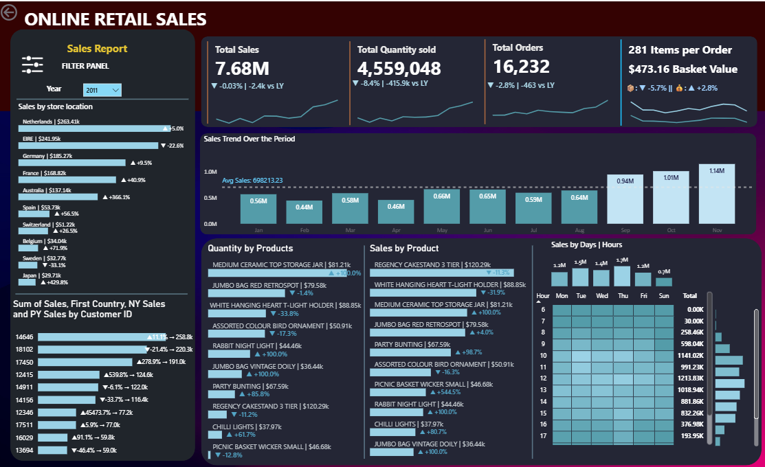
Online Retail Sales Analysis Dashboard

This project implemented a complete end-to-end data pipeline for the Online Retail II dataset, from ingestion and cleaning to analysis and visualization. The process transformed raw transactional data into actionable business insights through ETL processes, SQL analysis, and an interactive Power BI dashboard focused on year-over-year comparison between 2010 and 2011. The final deliverables provide stakeholders with clear insights into sales performance, customer behavior, and product trends to support data-driven decision making.

Goals:

• Ingest the Online Retail II dataset into MS SQL Server reliably despite its size (~1M rows)
• Create a cleaned, analysis-ready table named retail_data_cleaned
• Build a Power BI model with DAX measures to support YOY analysis
• Deliver interpretable insights and prioritized actions for stakeholders

Scope:

• Focused on transactions between Dec 1, 2009 and Dec 9, 2011, with primary comparison between 2010 and 2011
• Excluded deep supply-chain costing (COGS), external marketing data, and per-item supplier data

Dataset: Online Retail II (UCI Machine Learning Repository) — transactions of a UK online retailer

Columns (raw): InvoiceNo, StockCode, Description, Quantity, InvoiceDate, UnitPrice, CustomerID, Country

Record count: ~1,067,371 rows

Key Notes:

• Some invoices begin with C or A indicating cancellations or adjustments
• StockCode uses 5-digit patterns with exceptions (letters, short codes)
• CustomerID contains zeros to indicate missing customers
• Negative quantities exist (returns) and Price=0 rows (likely postage or data issues)

Business model: Non-store, UK online retailer selling giftware across global customers (retail + wholesalers)

Key assumptions made during cleaning:

• Invoices starting with non-numeric patterns are adjustments/cancellations
• CustomerID = 0 indicates anonymous or missing customer
• StockCodes must begin with 5 digits; others are dropped or flagged
• Rows with UnitPrice = 0 are data-noise and were removed after inspection

Environment:

• Local Windows development machine with Python 3.10+
• MS SQL Server Express
• Power BI Desktop (current stable release)

Key packages:

• pandas >= 1.5.0
• pyodbc >= 4.0.30
• numpy

ODBC driver:

• ODBC Driver 17 for SQL Server or later

File structure:

/OnlineRetailProject/
  ├─ data/
  │    └─ online_retail_II.csv
  ├─ notebooks/
  │    └─ Import Dataset from CSV to SQL.ipynb
  ├─ sql/
  │    ├─ create_tables.sql
  │    ├─ cleaning_queries.sql
  │    └─ analysis_queries.sql
  ├─ powerbi/
  │    └─ OnlineRetail_Dashboard.pbix
  ├─ docs/
  │    └─ Online Retail II — Full Project Documentation.md
  └─ scripts/
       └─ import_to_sql.py

Purpose: Reliably import the large CSV into MS SQL Server with robust type coercion and chunked inserts

Key patterns used:

• pandas.read_csv() with default streaming into memory
• pyodbc with cursor.fast_executemany = True for fast batched inserts
• Chunked executemany (50k rows per chunk) with commit per chunk and error capture

Python code (condensed example):

import pyodbc
import pandas as pd

# 1) Read CSV
csv_path = r"path\to\online_retail_II.csv"
df = pd.read_csv(csv_path)
print('Total rows to insert:', len(df))

# 2) Preprocessing
df['InvoiceDate'] = pd.to_datetime(df['InvoiceDate'], errors='coerce')
df['Quantity'] = pd.to_numeric(df['Quantity'], errors='coerce').fillna(0).astype(int)
df['Price'] = pd.to_numeric(df['UnitPrice'], errors='coerce').fillna(0.0)
df['CustomerID'] = df['CustomerID'].replace(0, pd.NA)
df['Description'] = df['Description'].astype(str).str.strip()

# 3) Connect to SQL
conn = pyodbc.connect(
    Driver='ODBC Driver 17 for SQL Server',
    Server=r'YUU\SQLEXPRESS',
    Database='online_retail',
    Trusted_Connection='yes',
    autocommit=False
)
cur = conn.cursor()
cur.fast_executemany = True

# 4) Prepare statement
sql = '''INSERT INTO dbo.invoices (Invoice, StockCode, Description, Quantity, InvoiceDate, Price, Customer_ID, Country) 
         VALUES (?,?,?,?,?,?,?,?)'''
params = df[['Invoice','StockCode','Description','Quantity','InvoiceDate','Price','CustomerID','Country']].values.tolist()

# 5) Chunked insert
chunk_size = 50000
for start in range(0, len(params), chunk_size):
    chunk = params[start:start+chunk_size]
    try:
        cur.executemany(sql, chunk)
        conn.commit()
        print(f'Committed rows {start}–{start+len(chunk)-1}')
    except Exception as e:
        print(f'Error inserting rows {start}–{start+len(chunk)-1}: {e}')
        pd.DataFrame(chunk).to_csv(f'failed_chunk_{start}.csv', index=False)
        break

cur.close()
conn.close()

Target table (cleaned workspace): dbo.retail_data_cleaned

Example CREATE TABLE for initial invoices:

CREATE TABLE dbo.invoices (
    Invoice VARCHAR(20),
    StockCode VARCHAR(50),
    Description VARCHAR(255),
    Quantity INT,
    InvoiceDate DATETIME2(0),
    Price DECIMAL(10,2),
    [Customer ID] VARCHAR(50),
    Country VARCHAR(50)
);

Safe copy creation:

SELECT * INTO dbo.retail_data_cleaned FROM dbo.retail_data;

Important indexed columns (recommended):

• Non-clustered index on InvoiceDate for time-based queries
• Index on StockCode to speed SKU aggregations
• Clustered index on a surrogate key for large OLTP workloads

1. Make a copy — to avoid destructive edits

   SELECT * INTO dbo.retail_data_cleaned FROM dbo.retail_data;

2. Remove placeholder customer IDs (0 → NULL)

   UPDATE dbo.retail_data_cleaned
   SET [Customer ID] = NULL
   WHERE [Customer ID] = 0;

3. Drop invoices that aren't standard orders

   DELETE FROM dbo.retail_data_cleaned
   WHERE Invoice NOT LIKE '[0-9][0-9][0-9][0-9][0-9][0-9]';

4. Remove non-standard StockCodes

   DELETE FROM dbo.retail_data_cleaned
   WHERE StockCode NOT LIKE '[0-9][0-9][0-9][0-9][0-9]%';

5. Convert negative quantities to positive (ABS)

   UPDATE dbo.retail_data_cleaned
   SET Quantity = ABS(Quantity);

6. Remove zero-priced rows

   DELETE FROM dbo.retail_data_cleaned
   WHERE Price = 0;

7. Normalize Description casing

   UPDATE dbo.retail_data_cleaned
   SET Description = CONCAT(UPPER(LEFT(Description,1)), LOWER(SUBSTRING(Description,2,LEN(Description))))
   WHERE Description IS NOT NULL;

8. Trim whitespace

   UPDATE dbo.retail_data_cleaned
   SET Description = LTRIM(RTRIM(Description))
   WHERE Description IS NOT NULL;

9. InvoiceDate normalization

   ALTER TABLE dbo.retail_data_cleaned ADD InvoiceDate_Converted DATETIME2(0);
   UPDATE dbo.retail_data_cleaned
   SET InvoiceDate_Converted = DATEADD(SECOND, DATEDIFF(SECOND, '1900-01-01', InvoiceDate), '1900-01-01');
   ALTER TABLE dbo.retail_data_cleaned DROP COLUMN InvoiceDate;
   EXEC sp_rename 'dbo.retail_data_cleaned.InvoiceDate_Converted','InvoiceDate','COLUMN';

10. Create date & time columns

    ALTER TABLE dbo.retail_data_cleaned
    ADD InvoiceDateOnly DATE, InvoiceTimeOnly TIME;
    UPDATE dbo.retail_data_cleaned
    SET InvoiceDateOnly = CAST(InvoiceDate AS DATE), InvoiceTimeOnly = CAST(InvoiceDate AS TIME);

11. Compute derived columns (Revenue/Sales)

    ALTER TABLE dbo.retail_data_cleaned
    ADD Sales AS (Price * Quantity);

12. Final QA counts

    SELECT COUNT(*) AS TotalRows FROM dbo.retail_data_cleaned;
    SELECT SUM(CASE WHEN Price=0 THEN 1 ELSE 0 END) AS ZeroPriceCount FROM dbo.retail_data_cleaned;
    SELECT (1.0 - CAST((SELECT COUNT(*) FROM dbo.retail_data_cleaned) AS FLOAT) / (SELECT COUNT(*) FROM dbo.retail_data)) * 100 AS TotalDataLossPercent;

Columns added/derived:

• Sales = Price * Quantity (calculated column)
• InvoiceDate split into InvoiceDate (date only) and InvoiceTime (time only)
• Hour = HOUR(InvoiceTime) for hourly analysis
• InvoiceDayOfWeek, InvoiceWeek, Month, Year

SQL examples:

ALTER TABLE dbo.retail_data_cleaned ADD InvoiceDate DATE;
ALTER TABLE dbo.retail_data_cleaned ADD InvoiceTime TIME;
UPDATE dbo.retail_data_cleaned
SET InvoiceDate = CAST(InvoiceDate AS DATE), InvoiceTime = CAST(InvoiceDate AS TIME);

-- Hour (SQL Server)
ALTER TABLE dbo.retail_data_cleaned ADD [Hour] AS DATEPART(HOUR, InvoiceTime);

Checks performed:

• Row counts before/after each major step
• Count of Price = 0 rows and manual inspection
• Verify Customer ID null counts
• Histogram / counts of StockCode lengths
• Spot-check top Description frequencies

SQL examples:

SELECT COUNT(*) FROM dbo.retail_data; -- original
SELECT COUNT(*) FROM dbo.retail_data_cleaned; -- cleaned
SELECT Description, COUNT(*) AS Frequency FROM dbo.retail_data_cleaned GROUP BY Description ORDER BY Frequency DESC;
SELECT LEN(StockCode) AS StockCodeLength, COUNT(*) AS Cnt FROM dbo.retail_data_cleaned GROUP BY LEN(StockCode) ORDER BY StockCodeLength;

Data model:

• Fact: retail_data_cleaned (Sales, Quantity, Invoice, StockCode, CustomerID, Country, InvoiceDate)
• Dimension: Date Table (Date, Year, Month, Month Number, Month Year, Month Year N, Day Name, Weekday Number)

Date Table (DAX):

Date Table = CALENDAR(MIN(retail_data_cleaned[InvoiceDate]), MAX(retail_data_cleaned[InvoiceDate]))

Columns created on Date table:

• Month = FORMAT('Date Table'[Date],"mmm")
• Month Number = MONTH('Date Table'[Date])
• Month Year = FORMAT('Date Table'[Date],"yyyy mmm")
• Month Year N = FORMAT('Date Table'[Date],"yyyy mm")
• Day Name = FORMAT('Date Table'[Date],"ddd")
• Week Day Number = WEEKDAY('Date Table'[Date], 2)

Relationships:

• Date Table[Date] 1→* retail_data_cleaned[InvoiceDate]

Modeling tips:

• Set Date Table as the official Date Table using Mark as Date Table in Power BI
• Set sort-by column for Month Year using Month Year N to ensure correct ordering
• For categorical axes like Hour or Day Name, set X-Axis Type to Categorical to avoid gaps

Core KPIs:

Total Sales = SUM(retail_data_cleaned[Sales])
Total Orders = DISTINCTCOUNT(retail_data_cleaned[Invoice])
Total Quantity sold = SUM(retail_data_cleaned[Quantity])
Avg Basket Value = DIVIDE([Total Sales],[Total Orders])
Avg Items per Order = DIVIDE([Total Quantity sold],[Total Orders])

CY / PY / NY measures:

CY Sales = CALCULATE([Total Sales], VALUES('Date Table'[Year]))
PY Sales = CALCULATE([CY Sales], DATEADD('Date Table'[Date], -1, YEAR))
NY Sales = CALCULATE([CY Sales], DATEADD('Date Table'[Date], +1, YEAR))
CY Order = CALCULATE([Total Orders], VALUES('Date Table'[Year]))
PY Order = CALCULATE([CY Order], DATEADD('Date Table'[Date], -1, YEAR))
CY Quantity = CALCULATE([Total Quantity sold], VALUES('Date Table'[Year]))
PY Quantity = CALCULATE([CY Quantity], DATEADD('Date Table'[Date], -1, YEAR))

CY Sales =
VAR _Year = SELECTEDVALUE('Date Table'[Year])
RETURN
    CALCULATE(
        [Total Sales],
        FILTER(
            ALL('Date Table'),        
            'Date Table'[Year] = _Year
        )
    )

CY Sales = 
CALCULATE(
  [Total Sales],
  VALUES('Date Table'[Year])
)

Average & trend helpers:

Yearly Month Avg Sales = AVERAGEX(SUMMARIZE(ALLSELECTED('Date Table'), 'Date Table'[Month]), [Total Sales])
Daily Avg Sales = AVERAGEX(ALLSELECTED(retail_data_cleaned[InvoiceDate]), [Total Sales])

Color rules:

Color For columns = IF([Total Sales] > [Yearly Month Avg Sales], "Above Average", "Below Average")
Color For Daily Bars = IF([Total Sales] > [Daily Avg Sales], "Above Average", "Below Average")

CM/PM for MOM:

CM Sales = VAR selected_month = SELECTEDVALUE('Date Table'[Month])
         RETURN TOTALMTD(CALCULATE([Total Sales], 'Date Table'[Month] = selected_month), 'Date Table'[Date])
PM Sales = CALCULATE([CM Sales], DATEADD('Date Table'[Date], -1, MONTH))

MOM Growth & Diff Sales =
VAR month_diff = [CM Sales] - [PM Sales]
VAR mom = DIVIDE(month_diff, [PM Sales])
VAR sign = IF(month_diff > 0, "+", "")
VAR sign_trend = IF(month_diff > 0, "▲", "▼")
RETURN
IF(
    ISBLANK([PM Sales]) || [PM Sales] = 0,
    FORMAT(month_diff / 1000, "0.0k") & " vs LM",
    sign_trend & " " & sign & FORMAT(mom, "0.0%") & " | " & sign & FORMAT(month_diff / 1000, "0.0k") & " vs LM"
)

YOY & labeling:

YOY Growth & Diff Sales =
VAR year_diff = [CY Sales] - [PY Sales]
VAR yoy = DIVIDE(year_diff, [PY Sales])
VAR _sign = IF(year_diff > 0, "+", "")
VAR _sign_trend = IF(year_diff > 0, "▲", "▼")
RETURN
IF(
    ISBLANK([PY Sales]) || [PY Sales] = 0,
    FORMAT(year_diff / 1000, "0.0k") & " vs LY",
    _sign_trend & " " & _sign & FORMAT(yoy, "#0.00%" & " | " & _sign & FORMAT(year_diff / 1000, "0.0k")) & " vs LY"
)

Label for Product Type (Sales) =
VAR MostCommonDescription = MAXX(TOPN(1, VALUES(retail_data_cleaned[Description]), COUNTROWS(retail_data_cleaned), DESC), retail_data_cleaned[Description])
RETURN MostCommonDescription & " | " & FORMAT([Total Sales]/1000, "$0.00k")

Label for Store Location = SELECTEDVALUE(retail_data_cleaned[Country]) & " | " & FORMAT([Total Sales]/1000, "$0.00k")

PlaceHolder = 0
Items per Order Label = FORMAT(DIVIDE([Total Quantity Sold], [Total Orders]), "0") & " Items per Order"

Main Dashboard (Overview — YOY-first):

• Header row: KPI cards (Total Sales, Total Quantity Sold, Total Orders, Avg Basket Value, Avg Items per Order) with small line charts showing trend and YOY change labels
• Left vertical filter area: Year/Month slicer, Country slicer, Top N filter
• Middle top: DoD comparison of monthly averages with Yearly Month Avg Sales constant line
• Right top: Sales by Country (bar chart or map) with YOY indicators
• Middle row: Sales by Hour (bar) and Sales by Day (column) plus Heatmap (hours × weekday)
• Bottom row: Top 10 Customers by Sales and Top 10 Products by Sales/Quantity

December Data Adjustment:

• A page-level filter excludes December from all visual elements on the "Sales Trend Over the Period" page
• This ensures consistent period matching between 2010 and 2011 (January-November only)
• All YOY calculations now accurately reflect comparable time periods

Heatmap page:

• Matrix: Rows = Hour, Columns = Day Name, Values = Total Sales with gradient fill
• Tooltip page with MOM & YOY numbers

Product Insights page:

• Top/Bottom product tables with filters to switch between revenue/quantity
• Dynamic labels and interactive tooltips using PlaceHolder

Styling:

• Rectangle card color: #242635 (card background - dark)
• Wallpaper: gradient blue-pink
• Flag behind rectangles: #340202
• Minimal sans-serif font, consistent sizing, and icons for compact KPI labels

KPIs to monitor weekly: Total Sales, Total Orders, Conversion Rate (if web data available), AOV, Top 10 SKUs by revenue and quantity, New vs Returning buyers.

Stakeholders:

• CEO: high-level revenue & growth recommendations
• CFO: revenue breakdown & P&L sensitivity (requires future COGS data)
• CMO: campaign recommendations and A/B test designs
• COO: staffing & fulfillment alignment (hourly cadence findings)
• Data/BI team: ETL reliability and model maintenance

Deliverables:

• retail_data_cleaned table in online_retail DB
• Power BI workbook (OnlineRetail_Dashboard.pbix)
• Documentation and an automated ETL notebook (Import Dataset from CSV to SQL.ipynb)
• Appendix containing SQL queries and data dictionary

Runbook (manual):

1. Ensure CSV file is present in data/online_retail_II.csv
2. Open import_to_sql.py (or the Jupyter notebook) and run; verify pyodbc.drivers() includes ODBC Driver 17
3. After import, run cleaning_queries.sql in SSMS, but operate on a copy (SELECT * INTO retail_data_cleaned FROM dbo.retail_data)
4. Open Power BI file and refresh data model

Automating:

• Convert notebook script into a scheduled task (Windows Task Scheduler) or job (SQL Agent if available) that runs nightly to import new data
• Add logging — each run should archive source CSV and record counts/rows inserted/failed

Top descriptions:

SELECT Description, COUNT(*) AS Frequency 
FROM dbo.retail_data_cleaned 
GROUP BY Description 
ORDER BY Frequency DESC;

StockCode length distribution:

SELECT LEN(StockCode) AS StockCodeLength, COUNT(*) AS Count 
FROM dbo.retail_data_cleaned 
GROUP BY LEN(StockCode) 
ORDER BY StockCodeLength;

Hourly sales heatmap source:

SELECT DATEPART(HOUR, InvoiceTime) AS Hour, 
       DATENAME(WEEKDAY, InvoiceDate) AS DayName, 
       SUM(Sales) AS TotalSales
FROM dbo.retail_data_cleaned
GROUP BY DATEPART(HOUR, InvoiceTime), DATENAME(WEEKDAY, InvoiceDate);

• Python 3.10+
• pandas >= 1.5.0
• pyodbc >= 4.0.30
• ODBC Driver 17 for SQL Server
• Power BI Desktop (stable 2025 release recommended)

Why MySQL? MySQL (and MariaDB) are open-source RDBMS with good tooling for imports (LOAD DATA INFILE) and broadly used in web stacks.

Possible benefits: Faster local CSV imports, flexible open-source tooling, easier cloud migration to managed MySQL engines.